In accordance with this formula, the price level is determined by the formula: P=MV/Q

The amount of money in circulation (money supply) M = PQ / V

Based on this formula, Fisher concludes that the value of money is inversely proportional to its quantity. Fisher's formula MV = PQ makes it possible to explain the phenomenon of inflation in terms of violations in the sphere of paper money circulation. Economic interpretation of the formula M = PQ/V: the more national product created in the country, the more money should be in circulation. With an increase in the physical quantity of goods and the prices of these goods, the money supply has to be increased, and, conversely, as the quantity of goods and prices for them decrease, the money supply must be narrowed. Under conditions of inflation, the amount of money in circulation is sensitive to the price level. For the normal functioning of commodity circulation and money circulation, it is necessary to increase the money supply in accordance with the rise in prices. Failure to comply with this principle leads to failures in the functioning of the commodity-money system, a shortage of money in circulation. State control over the money supply is necessary in order to influence prices, production, and the economy as a whole.

Wikimedia Foundation. 2010 .

See what the "Fischer formula" is in other dictionaries:

A stable distribution in probability theory is a distribution that can be obtained as a limit on the distribution of sums of independent random variables. Contents 1 Definition 2 Remarks 3 Properties of stable distributions ... Wikipedia

Fisher's exact test is a statistical significance test used in the analysis of contingency tables for small sample sizes. Named after its inventor R. Fisher. Refers to accurate tests significance, because not ... ... Wikipedia

A formula that sets the ratio between the change in bank interest rates and the change in spot exchange rates. According to the international Fisher effect, the difference in interest rates between two countries should be an unbiased predictor of the future... ... Financial vocabulary

FISHER DISTRIBUTION- is an analogue of the normal distribution on the sphere. R. Fisher's statistics is widely used in the processing of paleomagnetic data. Checking the compliance of the real distributions of the vectors Jn and its components with the Fisher distribution helps to evaluate ... ... Paleomagnetology, petromagnetology and geology. Dictionary reference.

Asymptotic expansion of the difference between the corresponding quantiles of the normal distribution and any distribution close to it in powers of a small parameter; studied by E. Cornish and R. Fisher. If F(x, t) is a distribution function,… … Mathematical Encyclopedia

Economics of a country- (National economy) The country's economy is public relations to ensure the wealth of the country and the well-being of its citizens The role of the national economy in the life of the state, the essence, functions, sectors and indicators of the country's economy, the structure of countries ... ... Encyclopedia of the investor

The purchasing power of money: its definition and relation to credit, interest and crises (eng. The Purchasing Power of Money: Its determination and relation to credit, interest and crises, 1911) is a work of the American economist I. Fisher. ... ... Wikipedia

Interest rate- (Interest rate) The interest rate is the percentage of monetary profit that the borrower pays to the lender for the money capital taken on a loan Determination of the interest rate, types of interest rates on loans, real and nominal interest ... ... Encyclopedia of the investor

Z-transform- Formula for transforming a sample of r values ​​(correlation coefficient) in order to approximate them to a normal distribution. Also called the Z Fisher transform... Dictionary in psychology

Correlation coefficient- (Correlation coefficient) The correlation coefficient is a statistical indicator of the dependence of two random variables Definition of the correlation coefficient, types of correlation coefficients, properties of the correlation coefficient, calculation and application ... ... Encyclopedia of the investor

Regulation of the amount of money in circulation and the price level is one of the main methods of influencing the economy.

The relationship between the quantity of money and the price level was formulated by representatives of the quantity theory of money.

In a free market () it is necessary to regulate economic processes to a certain extent (Keynesian model). The regulation of economic processes is carried out, as a rule, either by the state or by specialized bodies. As the practice of the 20th century has shown, many other important economic parameters depend on the one used in the economy, primarily the price level and interest rate (credit prices). The relationship between the price level and the amount of money in circulation was clearly formulated within the framework of the quantity theory of money.

Fisher's equation

Prices and the amount of money are directly related.

Depending on various conditions, prices may change due to changes in the money supply, but the money supply can also change depending on changes in prices.

The exchange equation looks like this:

Fisher formula

Undoubtedly, this formula is purely theoretical and unsuitable for practical calculations. Fisher's equation does not contain any single solution; within the framework of this model, multivariance is possible. However, under certain tolerances, one thing is certain: The price level depends on the amount of money in circulation. Usually two assumptions are made:

• the rate of money turnover is a constant value;
• All production capacities on the farm are fully utilized.

The meaning of these assumptions is to eliminate the influence of these quantities on the equality of the right and left sides of the Fisher equation. But even if these two assumptions are met, it cannot be unconditionally asserted that the growth of the money supply is primary, and the rise in prices is secondary. The dependence here is mutual.

In the conditions of stable economic development the money supply acts as a regulator of the price level. But with structural disproportions in the economy, a primary change in prices is also possible, and only then a change in the money supply (Fig. 17).

Normal economic development:

Disproportion of economic development:

Rice. 17. Dependence of prices on the money supply in conditions of stability or economic growth

Fisher formula (exchange equation) determines the amount of money used only as a medium of exchange, and since money also performs other functions, the determination of the total need for money involves a significant improvement in the original equation.

The amount of money in circulation

The amount of money in circulation and the total amount of commodity prices are related as follows:

The above formula was proposed by representatives quantitative theory of money. The main conclusion of this theory is that in each country or group of countries (Europe, for example) there must be a certain amount of money corresponding to the volume of its production, trade and income. Only in this case will the price stability. In the case of an inequality in the quantity of money and the volume of prices, changes in the price level occur:

In this way, price stability- the main condition for determining the optimal amount of money in circulation.

(this situation is typical for countries with developed market economies) they also use an approximate version of the Fisher formula.

What determines the Fisher formula

What value in the Fisher formula is called the inflationary premium

In what cases can you use an approximate version of the Fisher formula

Who is more profitable to use an approximate version of the Fisher formula in the contract for the lender or the borrower

Solution. To determine the desired interest rate, we use the Fisher formula (111) with r = 0.16 and h = OD

Note that when solving this example, formula (46) could also be used. Obviously, the Fisher formula also allows us to answer the questions of the example. In particular, substituting into it the values ​​of the interest rate and inflation of the first case (in the notation of the Fisher formula F = 0.45, /r = OD5), we obtain the equation 0.45 = r + OD5 + 0.15r, whence

Using the Fisher formula, determine the real profitability of a financial transaction if the interest rate on deposits for 12 months is 15%, and the annual inflation rate is 10%.

A more accurate relationship between interest rates and inflation is provided by Fisher's formula.

The results of such calculations can vary significantly. One of the methods for obtaining a single result is to construct a geometric mean of two territorial indices of the physical volume of production (Fischer's formula)

For task No. 8, we introduce the condition that the annual real interest rate was 80%, and the nominal one increased to 250%. Determine the inflation rate (to complete the task, find in the sources educational literature expression of the Fisher formula).

To avoid unreasonably high interest payments, it can be recommended when concluding loan agreements to provide for a revision of the interest rate depending on inflation. One of the possibilities of this kind is to fix in the loan agreement not a nominal, but a real interest rate (see Appendix 1), in order to increase it (according to the Fisher formula) in the calculation and payment of interest in accordance with the inflation that actually took place during this time .

Calculate the price and volume indices using the Fisher formula

Fisher did not find a perfect formula; there was not a single average that simultaneously met the proposed tests. However, this only confirmed his initial assumption that there is no ideal formula for the average index. The best was the formula, which is a combination of the Laspeyres and Paasche indices. It is called the ideal Fisher index.

What then lies main reason obtaining strange results when calculating according to different formulas, Fisher argued that the main errors accumulate at the stage of grouping goods into aggregated groups.

Fisher's formula is incorrect under the gold standard because it ignores the intrinsic value of money. However, when paper money is in circulation, which cannot be exchanged for gold, it acquires a certain meaning. Under these conditions, a change in the money supply affects the level of commodity prices, although, of course, I. Fischer idealized the price mechanism to a certain extent, since he assumed absolute elasticity of commodity prices. Fisher, like other neoclassicists, proceeded from perfect competition and extended his conclusions to a society in which monopolies dominated and prices had already largely lost their former elasticity.

The new equation of exchange is a variation of the quantity theory of money and therefore shares all its advantages and disadvantages. Of course, means of payment are an organic component of the modern money supply, however, it follows from the Fisher formula that they directly and directly affect commodity prices, which is not true.

M/P)° = /.(/, Y), since with an increase in income Y, the accumulated wealth of the individual W increases, and the Fisher formula / = r + jf tells us that with an increase in the inflation rate, nominal interest(opportunity cost of holding liquidity) and, accordingly, the demand for money falls.

Fisher's formula makes sense only with a gold coin standard; when switching to paper money circulation, it loses its meaning (yes).

Fisher's formula - the so-called ideal formula involves the calculation of the stock index using the geometric mean of the indices calculated on the basis of the Laspey-Rese and Paasche formulas.

West enjoy mathematical formula, proposed by the American economist I. Fisher, showing the dependence of the price level on the money supply MV = PQ, where M is the money supply V is the velocity of money P is the level of commodity prices Q is the number of circulating goods. In accordance with this formula, the level of commodity prices is determined by the formula / == Ml f/Q, i.e. the product of the mass of banknotes by the speed -Ax of circulation, divided by the number of goods, the volume of money mabs M = PQ / F. Based on this formula, Fisher concludes that the value of money is inversely proportional to its quantity. I. Fisher's equation of exchange MV = PQ expresses quantitative dependencies between the sum of commodity prices and the circulating money supply.

This formula more accurately reflects the effectiveness of investing funds in GKOs with their subsequent reinvestment over the entire 1 year, but only under conditions of a stable market and little changing prices for bonds of each issue. With inflation and fluctuations in interest rates, the real rate of return of a particular GKO issue can be calculated using the Fisher formula considered earlier

For understanding Fisher's concept, it is very important that the author formed it in order to find easy way and quick calculation of indices, and one of the informal requirements for the index formula, Fisher considered the following index to be simple and understandable for the uninitiated.

There are quite a few errors associated with the calculation of inflation. Shares, the most common of them, is the calculation of inflation not according to the Fisher formula, but according to the approximate formula K - N-I. Let's look at an example of what this leads to at various levels of inflation.

Let's touch upon such a complex economic term as the discount rate, consider the existing modern methods of its calculation and directions of use.

The discount rate and its economic meaning

Discount rate (analogue: comparison rate, rate of return) is the interest rate that is used to revalue future capital at the current moment. This is done because one of the fundamental laws of economics is the constant depreciation of the value (purchasing power, cost) of money. The discount rate is used in investment analysis when an investor decides on the prospect of investing in a particular object. To do this, he leads the future value of the investment object to the present (current). Conducting comparative analysis, he can decide on the attractiveness of the object. Any value of an object is always relative, so the discount rate is the very basic criterion with which the investment efficiency is compared. Depending on various economic tasks, the discount rate is calculated in different ways. Consider the existing methods for estimating the discount rate.

Methods for estimating the discount rate

Let's consider 10 methods for estimating the discount rate for evaluating investments and investment projects of an enterprise/company.

• CAPM Capital Asset Valuation Models;
• Modified CAPM Capital Asset Valuation Model;
• Model by E. Fama and K. French;
• Model M. Carhart;
• Constant Growth Dividend Model (Gordon);
• Calculation of the discount rate based on the weighted average cost of capital (WACC);
• Calculation of the discount rate based on return on equity;
• Market multiplier method
• Calculation of the discount rate based on risk premiums;
• Calculation of the discount rate based on expert assessment;

Calculation of the discount rate based on the CAPM model

Capital asset valuation model - CAPM ( CapitalassetPricingModel) was proposed in the 1970s by W. Sharp (1964) to estimate the future return on shares/capital of companies. The CAPM reflects future returns as a risk-free return and a risk premium. As a result, if the expected return on a stock is lower than the required return, investors will refuse to invest in this asset. The factor that determines the future rate in the model was taken as market risk. The formula for calculating the discount rate for the CAPM model is as follows:

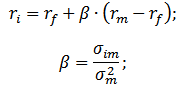where: r i – expected return on shares (discount rate);

r f is the yield on a risk-free asset (for example: government bonds);

r m - market return, which can be taken as the average return on the index (MICEX, RTS - for Russia, S & P500 - for the USA);

β is the beta coefficient. It reflects the riskiness of an investment in relation to the market, and shows the sensitivity of changes in stock returns to changes in market returns;

σ im is the standard deviation of the change in stock return depending on the change in market return;

σ 2 m is the dispersion of the market return.

Advantages and Disadvantages of the CAPM Capital Asset Pricing Model

• The model is based on the fundamental principle of linking stock return to market risk, which is its advantage;
• The model includes only one factor (market risk) to estimate the future performance of a stock. Researchers such as Y. Fama, K. French and others introduced additional parameters into the CAPM model to increase its forecasting accuracy.
• The model does not take into account taxes, transaction costs, stock market opacity, etc.

Calculation of the discount rate according to the modified CAPM model

The main disadvantage of the CAPM model is its single-factor approach. Therefore, adjustments for unsystematic risk are also included in the modified capital asset pricing model. Unsystematic risk is also called specific risk, which occurs only under certain conditions. Formula for calculating the modified CAPM model (modifiedCapitalassetPricingModel ,MCAPM) is as follows:

where: r i – expected return on shares (discount rate); r f is the yield on a risk-free asset (for example, government bonds); r m – market profitability; β is the beta coefficient; σ im is the standard deviation of the change in stock return from the change in market return; σ 2 m is the dispersion of market returns;

r u is the risk premium, which includes the non-systematic risk of the company.

As a rule, experts are used to assess specific risks, because they are difficult to formalize by means of statistics. The table below shows the various risk adjustments ⇓.

Specific risks	Risk adjustment, %
State influence on tariffs	0,4%
Changes in prices for raw materials, materials, energy, components, rent	0,2%
Management risk of the owner/shareholders	0,2%
Influence of key suppliers	0,3%
Influence of seasonality of demand for products	0,4%
Conditions for raising capital	0,3%
In total, the adjustment for specific risk is:	1,8%

For example, let's calculate the adjusted discount rate, so if the CAPM model returns 10%, then the risk-adjusted discount rate will be 11.8%. Using the modified model allows you to more accurately determine the future rate of return.

Calculation of the discount rate according to the model of E. Fama and K. French

One of the modifications of the CAPM model was the three-factor model of E. Fama and K. French (1992), which began to take into account two more parameters that affect the future rate of return: company size and industry specifics. Below is the formula for the three-factor model by E. Fama and K. French:

where: r – discount rate; r f is the risk-free rate; r m – profitability of the market portfolio;

SMB t is the difference between the returns of the weighted average portfolios of shares of small and large capitalization;

HML t is the difference between the returns of weighted average stock portfolios with large and small ratios of book value to market value;

β, si, h i - coefficients that indicate the influence of parameters r i , r m , r f on the profitability of the i-th asset;

γ is the expected profitability of the asset in the absence of the influence of 3 risk factors on it.

Calculation of the discount rate based on the model of M. Karhat

The three-factor model of E. Fama and K. French was modified by M. Carhart (1997) by introducing the fourth parameter to assess the possible future profitability of a stock - the moment. The moment reflects the rate of price change over a certain historical period of time, when the fourth parameter is used in the model for assessing the profitability of a stock in the future, it is taken into account that the rate of price change also affects the future rate of return. Below is the formula for calculating the discount rate according to the M. Carhart model:

where: r – discount rate; WMLt - the moment, the rate of change in the value of the stock for the previous period.

Calculation of the discount rate based on the Gordon model

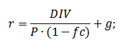
Another method for calculating the discount rate is to use the Gordon model (Constant Growth Dividend Model). This method has some restrictions on its use, because in order to estimate the discount rate, it is necessary that the company issues ordinary shares with dividend payments. Below is the formula for calculating the cost of equity of an enterprise (discount rate):

where:

DIV is the amount of expected dividend payments per share per year;

P is the placement price of shares;

fc is the cost of issuing shares;

g is the growth rate of dividends.

Calculation of the discount rate based on the weighted average cost of capital WACC

Method for estimating the discount rate based on the weighted average cost of capital (eng. WACC, Weighted Average Cost of Capital) one of the most popular and shows the rate of return that should be paid for the use of investment capital. Investment capital can consist of two sources of financing: equity and debt. Often, WACC is used both in financial and investment analysis to assess the future return on investment, taking into account the initial conditions for the return (profitability) of investment capital. The economic meaning of calculating the weighted average cost of capital is to calculate the minimum allowable level of profitability (profitability, profitability) of the project. This indicator is used to evaluate the investment in an existing project. The formula for calculating the weighted average cost of capital is as follows:

where: r e ,r d is the expected (required) return on equity and borrowed capital, respectively;

E/V, D/V - share of own and borrowed capital. The sum of own and borrowed capital forms the capital of the company (V=E+D);

t is the income tax rate.

Calculation of discount rate based on return on equity

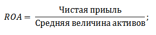
The advantages of this method lie in the possibility of calculating the discount rate for enterprises that are not listed on the stock market. Therefore, to assess the discount, indicators of return on equity and borrowed capital are used. These indicators are easily calculated by balance sheet items. If the company has both own and borrowed capital, then the indicator is used - return on assets (Return On Assets, ROA). The formula for calculating the return on assets is presented below:

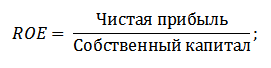
The next of the methods for estimating the discount rate through the return on equity (Return On Equity, ROE), which shows the efficiency/profitability of enterprise (company) capital management. The profitability ratio shows what rate of return the company creates at the expense of its capital. The formula for calculating the coefficient is as follows:

Developing this approach in assessing the discount rate through assessing the return on capital of an enterprise, a more accurate indicator can be used as a criterion for assessing the rate - the return on capital employed (ROCE,returnOnCapitalEmployed). This indicator, unlike ROE, uses long term duties(through shares). This indicator can be used for companies that have preferred shares in the stock market. If the company does not have them, then the ROE equals ROCE. The indicator is calculated by the formula:

Another variation of the return on equity ratio is the return on average capital employed ROACE (Return on Average Capital Employed).

In fact, this indicator corresponds to ROCE, its main difference lies in the averaging of the cost of capital employed (Equity + long-term liabilities) at the beginning and end of the estimated period. The formula for calculating this indicator:

ROACE can often replace ROCE, for example in the EVA formula. Let us analyze the feasibility of using profitability ratios to assess the discount rate ⇓.

Calculation of the discount rate based on expert judgment

If you want to estimate the discount rate for a venture project, then using the CAPM, Gordon model and WACC methods is impossible, so experts are used to calculate the rate. The essence of expert analysis lies in the subjective assessment of various macro, meso and micro factors that affect the future rate of return. Factors that have a strong influence on the discount rate: country risk, industry risk, production risk, seasonal risk, managerial risk, etc. For each individual project, experts identify their most significant risks and evaluate them using scores. The advantage of this method is the ability to take into account all the possible requirements of the investor.

Discount rate calculation based on market multiples

This method is widely used to calculate the discount rate for enterprises that have issues of ordinary shares in the stock market. As a result, the market multiple E/P is calculated, which translates as EBIDA/Price. The advantage of this approach lies in the fact that the formula reflects industry risks when evaluating a company.

Calculation of the discount rate based on risk premiums

The discount rate is calculated as the sum of the risk-free interest rate, inflation and risk premium. As a rule, this method of estimating the discount rate is carried out for various investment projects, where it is difficult to statistically assess the amount of possible risk / return. The formula for calculating the discount rate, taking into account the risk premium:

where:

r is the discount rate;

r f is the risk-free interest rate;

r p is the risk premium;

I is the percentage of inflation.

The discount rate formula consists of the sum of the risk-free interest rate, inflation, and risk premium. Inflation was singled out as a separate parameter, because the depreciation of money goes on constantly, this is one of the most important laws of the functioning of the economy. Let's consider separately how each of these components can be evaluated.

Methods for estimating the risk-free interest rate

To assess the risk-free one, such financial instruments are used that give profitability at zero risk, that is, absolutely reliable. In reality, no instrument can be considered absolutely reliable, just the probability of losing money when investing in it is extremely small. Consider two methods for estimating the risk-free rate:

1. Yield on risk-free government bonds (GKO - government short-term zero-coupon bonds, OFZ - federal loan bonds) issued by the Ministry of Finance of the Russian Federation. Government bonds have the highest reliability rating, so they can be used to calculate the risk-free interest rate. The yield on these types of bonds can be viewed on the website of the Central Bank of the Russian Federation (cbr.ru) and on average it can be taken as 6% per annum.
2. Yield on 30-year US bonds. The average yield on these financial instruments is 5%.

Methods for estimating the risk premium

The next component of the formula is the risk premium. Since risks always exist, their impact on the discount rate should be assessed. There are many methods for assessing the additional risks of an investment, let's consider some of them.

Methodology for assessing risk adjustments from Alt-Invest

Alt-Invest's methodology includes in the risk adjustment the following types of risks, presented in the table ⇓.

Methodology of the Government of the Russian Federation No. 1470 (dated 11/22/97) for estimating the discount rate for investment projects

The purpose of this methodology is to evaluate investment projects for public investment. Specific risk and adjustment for them will be calculated through expert assessment To calculate the basic (risk-free) discount rate, the refinancing rate of the Central Bank of the Russian Federation was used, this rate can be viewed on the official website of the Central Bank of the Russian Federation (cbr.ru). The specific risks of the project are assessed by experts in the presented ranges. The maximum discount rate for this method will be 61%.

Risk free interest rate
FROM refinancing rate of the Central Bank of the Russian Federation	11%
risk premium
Specific risks	Risk adjustment, %
Investments for the intensification of production	3-5%
Increasing product sales	8-10%
The risk of introducing a new type of product to the market	13-15%
R&D costs	18-20%

Methodology for calculating the discount rate Vilensky P.L., Livshits V.N., Smolyaka S.A.

Specific risks	Risk adjustment, %
1. The need to conduct R&D (with previously unknown results) by specialized research and (or) design organizations:
duration of R&D less than 1 year	3-6%
duration of R&D over 1 year:
a) R&D is carried out by one specialized organization	7-15%
b) R&D is complex and is carried out by several specialized organizations	11-20%
2. Characteristics of the applied technology:
Traditional	0%
New	2-5%
3. Uncertainty in the volume of demand and prices for manufactured products:
existing	0-5%
New	5-10%
4. Instability (cyclicality, seasonality) of production and demand	0-3%
5. Uncertainty of the external environment during the implementation of the project (mining and geological, climatic and other natural conditions, aggressiveness of the external environment, etc.)	0-5%
6. Uncertainty in the process of mastering the applied equipment or technology. The possibility for participants to ensure compliance with technological discipline	0-4%

Methodology for calculating the discount rate by Ya. Khonko for various classes of investments

The scientist Ya. Honko presented a methodology for calculating risk premiums for various classes of investments/investment projects. These risk premiums are presented in aggregate form, and the investor needs to choose the investment objective and, in accordance with it, the risk adjustment. Below are the aggregate risk adjustments depending on the purpose of the investment. As you can see, with an increase in the size of the risk, the ability of the enterprise / company to enter new markets, expand production and increase competitiveness also increases.

Summary

In this article, we looked at 10 methods for estimating the discount rate that use different approaches and assumptions in the calculation. The discount rate is one of the central concepts in investment analysis, it is used to calculate indicators such as: NPV, DPP, DPI, EVA, MVA, etc. It is used in estimating the value of investment objects, shares, investment projects, and management decisions. When choosing an assessment method, it is necessary to take into account for what purposes the assessment is made and what initial conditions. This will allow for the most accurate assessment. Thank you for your attention, Ivan Zhdanov was with you.

The concept of the discount rate is used to bring the future value to the present value. The discount rate is the interest rate used to convert future cash flows into one present value.

The calculation of the discount rate coefficient is carried out in different ways, depending on what task is set. And the heads of companies or individual departments in modern business are faced with completely different tasks:

• implementation of investment analysis;
• business planning;
• business valuation.

For all these areas, the basis is the discount rate (its calculation), since the definition of this indicator directly affects the decision-making regarding the investment of funds, the valuation of a company or certain types of business.

Discount rate from an economic point of view

Discounting determines the cash flow (its value) that relates to periods in the future (that is, future earnings in this moment). In order to correctly assess future income, it is necessary to have information about the forecasts of the following indicators:

• investments;
• expenses;
• revenue;
• capital structure;
• residual value of the property;
• discount rate.

The main purpose of the discount rate indicator is to evaluate the effectiveness of investments. This indicator implies the rate of return per 1 rub. invested capital.

The discount rate, the calculation of which determines the required amount of investments to receive future income, is a key indicator when choosing investment projects.

The discount rate reflects the value of money, taking into account time factors and risks. If we talk about the specifics, then this rate rather reflects an individual assessment.

An example of selecting investment projects using the discount rate factor

Two projects A and C are proposed for consideration. initial stage you need to invest 1000 rubles, there is no need for other costs. If you invest in project A, then you can earn an income of 1000 rubles annually. If you implement project C, then at the end of the first and second years the income will be 600 rubles, and at the end of the third - 2200 rubles. It is necessary to select a project, 20% per annum is the estimated discount rate.

Calculation of NPV (current value of projects A and C) is carried out according to the formula.

Ct - cash flows for the period from the first to the T-th years;

Co - initial investment - 1000 rubles;

r - discount rate - 20%.

NPV A \u003d - 1000 \u003d 1106 rubles;

NPV C \u003d - 1000 \u003d 1190 rubles.

So, it turns out that it is more profitable for the investor to choose project C. However, if the current discount rate were 30%, then the cost of the projects would be almost the same - 816 and 818 rubles.

This example demonstrates that the investor's decision fully depends on the discount rate.

Various methods for calculating the discount rate are proposed for consideration. In this article, they will be considered objectively in descending order.

Weighted average cost of capital

Most often, when conducting an investment calculation, the discount rate is determined as the weighted average cost of capital, taking into account the cost indicators of equity (equity) capital and loans. This is the most objective way to calculate the discount rate for cash flows. Its only drawback is that not all companies can practically use it.

In order to conduct a valuation of equity capital, the Long-Term Assets Valuation Model (CAPM) is used.

At the end of the 20th century, American economists John Graham and Campbell Harvey surveyed 392 directors and finance managers of enterprises in various fields of activity to determine how they make decisions, what they pay attention to in the first place. As a result of the survey, it was revealed that the most used academic theory, or rather, most firms calculate their equity capital using the CAPM model.

Cost of equity (calculation formula)

When calculating the cost of equity, the discount rate is considered otherwise.

Re - the rate of return, or, in other words, the discount rate of equity, is calculated as follows:

Re = rf + ?(rm - rf).

Where are the discount rate components:

• rf is the risk-free rate of return;
• ? - a coefficient that determines how the price of a firm's shares changes in comparison with changes in stock prices for all firms in a given market segment;
• rm - average market rate of return on the stock market;
• (rm - rf) - market risk premium.

AT different countries different approaches are chosen to determine the components of the model. Much in the choice depends on the general state attitude to calculation. Each of these indicators is important to study and understand separately, in this way cash flow can be determined. Therefore, the elements of the model "Valuation of long-term assets" will be considered in more detail below. And also the objectivity of each component was assessed and the discount rate was assessed.

Constituent Models

The rf is the rate of return on investment in risk-free assets. Risk-free assets are those in which the risk is zero when invested. These mainly include government securities. The calculation of discount rate risks varies from country to country. For example, in the United States, for example, treasury bills are classified as risk-free assets. In our country, for example, such assets are Russia-30 (Russian Eurobonds), the maturity of which is 30 years. Information on the yield of these securities is presented in most economic and financial publications, such as the newspaper Vedomosti, Kommersant, The Moscow Times.

The coefficient with a question mark in the model means sensitivity to changes in the systematic market risk of the return on securities of a particular firm. So, if the indicator is equal to one, then changes in the value of the shares of this company completely coincide with changes in the market. If ?-coefficient = 1.3, then it is expected that with a general rise in the market, the price of the shares of this company will rise 30% faster than the market. And vice versa accordingly.

In countries where the stock market is developed, the ?-coefficient is considered by specialized information and analytical agencies, investment and consulting companies, and this information is published in specialized periodicals that analyze stock markets and financial directories.

Rm - rf, which is the market risk premium, is the amount by which the average market rate of return on the stock market has long exceeded the rate of return on risk-free securities. Its calculation is based on statistical data on market premiums over a long period.

Calculating the weighted average cost of capital

If, when financing a project, not only own, but also borrowed funds are involved, then the income received from this project should compensate not only the risks associated with investing own funds, but also the funds spent on obtaining borrowed capital. To account for the cost of both equity and debt capital, the weighted average cost of capital is used, the calculation formula is below.

The CAPM model is used to calculate the discount rate. Re - rate of return on own (share) capital.

D is the market value of debt capital. Practically represents the amount of loans of the company according to the financial statements. If such data are not available, the standard ratio of equity to debt of similar firms is used.

E - market value of share capital (own capital). Obtained by multiplying the total number of shares of a common firm by the price of one share.

Rd represents the firm's rate of return on debt capital. These costs include information about bank interest on loans and bonds of a corporate type company. In addition, the valuation of borrowed capital is adjusted taking into account the income tax rate. Interest on credits and loans under tax legislation is attributed to the cost of goods, thus reducing the tax base.

Tc - income tax.

WACC Model: Calculation Example

The WACC model specifies a discount rate for Company X.

The calculation formula (its example was given when calculating the weighted average cost of capital) requires the following input indicators.

• Rf = 10%;
• ? = 0,90;
• (Rm - Rf) = 8.76%.

So, equity (its profitability) is equal to:

Re = 10% + 0.90 x 8.76% = 17.88%.

E / V = ​​80% - the share that the market value of equity capital takes in the total cost of capital of company X.

Rd = 12% - the weighted average level of costs for raising borrowed funds for company X.

D/V = 20% - the share of the company's borrowed funds in the total cost of capital.

tc = 25% - income tax indicator.

So WACC = 80% x 17.88% + 20% x 12% x (1 - 0.25) = 14.32%.

As noted above, certain methods for calculating the discount rate are not suitable for all companies. And this technique is exactly this case.

Firms are better off choosing other ways to calculate the discount rate if the company is not a public company and its shares are not traded on a stock exchange. Or if the company does not have enough statistics to determine the?-coefficient and it is impossible to find similar companies.

Cumulative assessment methodology

The most common and most often used method in practice is the cumulative method, with the help of which the discount rate is also estimated. The calculation by this method assumes the following conclusions:

• if investments did not imply risk, then investors would require a risk-free return on their capital (the rate of return would correspond to the rate of return on investments in risk-free assets);
• The higher the risk of the project is assessed by the investor, the higher the requirements for its profitability.

Therefore, when calculating the discount rate, the so-called risk premium must be taken into account. Accordingly, the discount rate will be calculated as follows:

R = Rf + R1 + ... + Rt,

where R is the discount rate;

Rf - risk-free rate of return;

R1 + ... + Rt - risk premiums for different risk factors.

It is practically possible to determine one or another risk factor, as well as the value of each of the risk premiums, only by expert means.

When determining the effectiveness of investment projects, the cumulative method for calculating the discount rate recommends taking into account 3 types of risk:

• the risk resulting from the dishonesty of the project players;
• risk resulting from non-receipt of planned income;
• country risk.

The value of the country risk is indicated in various ratings, which are compiled by special rating firms and consulting companies (for example, BERI). The fact of the unreliability of the project participants is compensated by a risk premium, the recommended indicator is no more than 5%. The risk arising as a result of not receiving the planned income is determined in accordance with the objectives of the project. There is a special calculation table.

Discount rates estimated by this method are quite subjective (too dependent on expert risk assessment). They are also much less accurate than the calculation methodology based on the Long-Term Assets Valuation model.

Expert assessment and other calculation methods

The simplest way to calculate the discount rate and quite popular in real life is the installation of its expert method, with reference to the requirements of investors.

It is clear that for private investors, calculation based on formulas cannot be the only way to make a decision regarding the correctness of setting the discount rate for a project/business. Any mathematical models can only approximately estimate the reality of the situation. Investors, relying on their own knowledge and experience, are able to determine a sufficient return for the project and rely on it as a discount rate when making calculations. But for adequate sensations, an investor must be very well versed in the market, have extensive experience.

However, it must be assumed that the expert method is the least accurate and may well distort the results of business (project) evaluation. Therefore, it is recommended that when determining the discount rate by expert or cumulative methods, it is mandatory to analyze the sensitivity of the project to changes in the discount rate. In this case, investors will have the most accurate assessment.

Of course, there are alternative ways to calculate the discount rate. For example, the theory of arbitrage pricing, the model of dividend growth. But these theories are very difficult to understand and are rarely applied in practice.

Applying the discount rate in real life

In conclusion, I would like to note that most companies in the course of their activities need to determine the discount rate. It must be understood that the most accurate indicator can be obtained using the WACC methodology, while in other methods there is a significant error.

In work, it is not often necessary to calculate the discount rate. This is mainly due to the evaluation of large and significant projects. Their implementation entails a change in the capital structure, the company's share price. In such cases, the discount rate and method of its calculation are agreed with the investing bank. Focus mainly on the received risks in similar companies and markets.

The application of certain methods also depends on the project. In cases where industry standards, production technology, financing are understood and known, statistical data have been accumulated, the standard discount rate established by the enterprise is used. When evaluating small and medium projects, they refer to the calculation of payback periods, with an emphasis on the analysis of the structure and external competitive environment. In fact, methods for calculating the discount rate of real options and cash flows are combined.

You need to be aware that the discount rate is only an intermediate link in the evaluation of projects or assets. In fact, the assessment is always subjective, the main thing is that it be logical.

There is such a mistake - economic risks are taken into account twice. So, for example, two concepts are often confused - country risk and inflation. As a result, the discount rate is doubled, a contradiction appears.

It is not always necessary to count. There is a special table for calculating the discount rate, which is very easy to use.

Another good indicator is the cost of a loan for a particular borrower. The discount rate setting can be based on the actual lending rate and the level of yield of bonds that are available on the market. After all, the profitability of the project does not exist only within its own environment, it is also affected by the general economic situation on the market.

However, the obtained indicators also require significant adjustments related to the risk of the business (project) itself. Currently, the method of real options is quite often used, but it is very complicated from a methodological point of view.

In order to take into account such risk factors as the option of project suspension, changes in technology, market losses, discount rates (up to 50%) are artificially inflated by project appraisal practitioners. At the same time, there is no theory behind these figures. Similar results may well be obtained using complex calculations, in which, in any case, most of the predictive indicators would be determined subjectively.

Correctly determining the discount rate is a problem associated with the main requirement for the information content generated in financial reporting and accounting. In other words, if there is reason to doubt whether assets or liabilities are valued correctly, and not whether cash consideration is deferred, then discounting should be applied.

When choosing a discount rate, it is important to understand that it should be as close as possible to the rate received by the borrower of the lending bank on real terms in the existing environment.

So, the discount rate for certain assets (say, for fixed assets) is equated to the rate at which the firm would have to pay, raising funds to purchase similar property.